Tutorial and Recipes

In this tutorial we walk through each important class and function, and explain each one’s purpose and use with an example. At the end of the tutorial in Example: Parameter sensitivity we show a more advanced workflow involving parameter sensitivity over dual parameter space that uses several of the previously described classes and functions.

Data

The Data Class class loads a PRMS data file into a Pandas DataFrame and allows for easy modification and writing of PRMS data files.

A PRMS data file holds time series variables that are used as input for running PRMS, e.g. daily air temperature and precipitation. Being tabular and date-indexed the data file is well represented and managed as a pandas.DataFrame. A common paractice in hydrologic modeling is to evaluate hydrologic response to multiple climate change scenarios. The Data class offers function-based modification of time series variable/s so that the user can quickly create new climate inputs for PRMS. The user can visualize the data file variables from easily using Pandas, matplotlib or other plotting libraries. After modification of climatic variables the Data.write method will save the data to disk in the PRMS ascii format.

from prms_python import Data
d = Data('test/data/data')

# modify daily temperature by adding 2 degrees to each input
def f(x):
  return (x + 2)

# apply function to daily temperature input
d.modify(f, ['tmax','tmin'])

# write new modified data file to disk
d.write('test/data/temp_plus2_data')

The Data.data_frame property is the pandas.DataFrame representation of hydro-climatic variables found in a PRMS data file. As such it can also be assigned within Python. However in order to create a data file from scratch using the Data object one must also assign the Data.metadata property. For an example of what is stored in the metadata attribute please refer to the data examples Jupyter notebook.

The write method of data has dual functions depending on the status of a Data instance– if the method is called before the Data.data_frame is accessed then the original file will be simply copied to the path given to write, on the other hand if the data_frame has been accessed within Python then the write method writes the current state of the data in the data_frame from memory. The first function is useful in reducing memory use and computational cost when using the Data class in more advanced workflows.

The Scenario and ScenarioSeries will soon incorporate the functionality to modify the climatic data within either a single Scenario or a series of Scenarios.

Parameters

The Parameters Class provides a NumPy-backed representation of a PRMS parameters file that allows the user to select, modify, and save PRMS parameters files. It can be used similarly to a Pandas DataFrame.

The PRMS parameters file contains data arrays of varying dimensionality, which is why we can’t simply use a DataFrame to do these manipulations. The implementation of the Parameters class is loosely based on the netCDF data structure, where metadata about each parameter is kept separately. Parameters are read into memory only if the user selects or modifies a particular parameter. This allows for memory-efficient processing of Parameter files.

Below is an example of reading a parameter file, reading a particular variable from a parameter file, replacing that parameter data with other data (in this case an array of all zeros), then saving the modified parameters to a new Parameters file.

from prms_python import Parameters
p = Parameters('test/data/parameter')

# select PRMS parameter by name, raising KeyError if DNE
snow_adj = p['snow_adj']
assert snow_adj.shape == (12, 16)

# assign values to PRMS parameter
import numpy as np
z = np.zeros(snow_adj.shape)
p['snow_adj'] = z  # now p['snow_adj'] is 12x16 matrix of zeros

# write modified parameters to file
p.write('newparameters')

The Scenario and ScenarioSeries use this functionality (via the prms_python.modify_params function) to implement either a single Scenario or a series of Scenarios.

Simulation & SimulationSeries

The Simulation class provides a simple wrapper around running the PRMS model. It encourages standardization of input file names by requiring the three PRMS inputs to be named data, parameters, and control. In order to add some natural metadata to the inputs, the user should use a memorable name for the directory that holds these three files. The Simulation and SimulationSeries however are more useful as building blocks for more advanced workflows or for new PRMS-Python submodules and routines, e.g. new optimization routines.

After the user prepares their input files, say into a directory called prms-sim-example, they can run the following in either a Python script or a Python REPL

from prms_python import Simulation
sim = Simulation('prms-sim-example')
sim.run()

This will run PRMS assuming the PRMS executable is on the system path and is called prms. In this usage, the outputs will go to the prms-sim-dir directory. If the user wishes to use a different executable name or provide the path to it explicitly, they can do so by replacing

sim.run()

with

sim.run(prms_executable='path/to/myPRMSExecutable')

Another available option is to specify a different directory to use as the “simulation directory,” which can be useful if you want to separate a directory with only input data from directories where both input and output model run data will be stored. You can do this by specifying an additional keyword argument in the Simulation constructor, like so

sim = Simulation('prms-sim-example', simulation_dir='sim-dir-1')
sim.run()

Additional examples of Simulation including the file structure can be found in the API prms_python.Simulation.run() and the class method from_data which allows for initialization from PRMS-Python Data and Parameter objects can be found in the API at prms_python.Simulation.from_data().

SimulationSeries

The SimulationSeries class offers the same functionality as Simulation for an arbitrary number of simulations, with the added function of running PRMS in parralel. The example below is taken from the PRMS-Python API.

Lets say you have already created a series of PRMS models by modifying the input climatic forcing data, e.g. you have 100 data files and you want to run each using the same control and parameters file. For simplicity lets say there is a directory that contains all 100 data files e.g. data1, data2, … or whatever they are named and nothing else. This example also assumes that you want each simulation to be run and stored in directories named after the data files as shown.

data_dir = 'dir_that_contains_all_data_files'
params = Parameters('path_to_parameter_file')
control_path = 'path_to_control'
# a list comprehension to make multiple simulations with
# different data files, alternatively you could use a for loop
sims = [
        Simulation.from_data
          (
            Data(data_file),
            params,
            control_path,
            simulation_dir='sim_{}'.format(data_file)
          )
        for data_file in os.listdir(data_dir)
        ]

Next we can use SimulationSeries to run all of these simulations in parrallel. For example we may use 8 logical cores on a common desktop computer.

sim_series = SimulationSeries(sims)
sim_series.run(nprocs=8)

The SimulationSeries.run() method will run all 100 simulations where chunks of 8 at a time will be run in parrallel. Inputs and outputs of each simulation will be sent to each simulation’s simulation_dir following the file structure of Simulation.run().

Scenario & ScenarioSeries

The Scenario class implements data management on top of the Simulation class, enforcing the user to separate base input data and simulation input and output data, plus simple, optional metadata. Let’s dive in with an example, assuming there are properly-formed files called data, control, and parameters, in a directory called base-inputs. We’ll use a simulation directory called sim-dir and further provide a title and description for the Scenario. If sim-dir exists it will be overwritten and if it does not exist it will be created. It’s up to the user to make sure data doesn’t get overwritten.

Both Scenarios and ScenarioSeries have a three-step process for set-up and run. First the Scenario or ScenarioSeries must be initialized with the base and simulation paths, plus, optionally, a title and description. Next, the Scenario(Series) must be “built”. This means defining which/how parameters should be modified.

Scenario

First, let’s see how we implement these three steps for a single Scenario. We’ll just increase one parameter, jh_coef, by 10%, or multiply by a scaling factor of 1.10.

sc = Scenario('base-inputs', 'sim-dir',
              title='Example Scenario',
              description='''
For the case of documentation we are including some example code.
Unless you actually have some inputs in the base-inputs directory used above
this will fail in an interpreter.
''')
def scale_1p1(x):
    return x * 1.1
sc.build({'jh_coeff': scale_1p1})
sc.run()

ScenarioSeries

Now let’s build and run a series of scenarios. Each Scenario in the series is specified by a dictionary that needs to have the title of the scenario and a key-value pair of parameter-function for every parameter that should be modified. In this example, we’ll still just scale jh_coef, but now over a range of values from 0.5 to 1.5, in increments of 0.1.

base_dir = '../models/lbcd/'
simulation_dir = 'example-sim-series-dir'
title = 'Jensen-Hays and Radiative Transfer Function Sensitivity Analysis'
description = '''
Use title of \'"jh_coef":{jh factor value}\' so later
we can easily generate a dictionary of these param/function combinations.
'''
sc_series = ScenarioSeries(base_dir, simulation_dir, title, description)

# define the scenario_list used to build the ScenarioSeries;
# build series in three steps:

#  1) define fun to return a function that scales a value by an amount
def _scale_fun(scale_val):
    def scale(x):
        return x * scale_val

    return scale
#  2) use the function generator `_scale_fun` in scenario_list comprehension
scenario_list = [
    {
        'title': '"jh_coef":{0:.1f}'.format(jh_val),
        'jh_coef': _scale_fun(jh_val),
    }
    for jh_val in np.arange(0.5, 1.5, 0.1)
]
#  3) "build" the series, meaning create scenario inputs and scenario dirs
sc_series.build(scenario_list)

sc_series.run()  # could provide nproc, ex: sc_series.run(nproc=10)

If, for example, we wanted to co-vary jh_coef with scalings of rad_trncf (or any other parameter) we can use the following as a recipe. Just add one more key/value pair to the dictionaries generated in the list comprehension that build the scenario_list.

scenario_list = [
    {
        'title': '"jh_coef":{0:.1f}|"rad_trncf":{1:.1f}'.format(jh_val, rad_val),
        'jh_coef': _scale_fun(jh_val),
        'rad_trncf': _scale_fun(rad_val)
    }
    for jh_val in np.arange(0.5, 1.5, 0.1)
    for rad_val in np.arange(0.5, 1.5, 0.1)
]

Note that this will square the number of scenarios to be done.

The title might look strange, but it is useful as part of the metadata to recover information about the individual Scenarios in the data analysis steps shown below in Example: Parameter sensitivity. Alternatively, if the title is omitted the subdirectory names of each scenario will not be intuitively matched to the unique universal identifiers that are assigned automatically by ScenarioSeries.build. However metadata for each scenario’s simulation will be stored in its respective directory and could later be used to refer which parameter(s) were modified and how because the metadata file contains a text representation of the Python functions that were used to modify the parameter(s).

Additional explanations and examples including the file structures and metadata created by the Scenario and ScenarioSeries are found in the API prms_python.Scenario and prms_python.ScenarioSeries.

Optimizer & OptimizationResult

The Optimizer class holds routines for PRMS parameter optimization or calibration, and sensitivity.uncertainty analysis. Currently the Optimizer.monte_carlo method offers a parameter resampling routine that can automate the resampling or an arbitrary number of PRMS parameters, conduct simulations for each set of resampled parameters, and self-generate metadata for each. The routine uses the stand-alone function prms_python.optimizer.resample_param which utilizes the uniform and normal distributions with added functionalities for parameters of varying dimensions. In other words there are different rules for parameter resampling for spatial parameters or parameters of large dimension than those of single value or monthly dimensions.

The OptimizationResult class is designed to aid management and analysis of output from a single optimization stage.

Note, this section is currently under development, please refer to the example Jupyter notebook here for detailed documentation of the monte_carlo parameter resampling routine. And the notebook here for explanations and examples for OptimizationResult.

load_data & load_statvar

Among other uses, if we want to compare the performance of our model to historical data for the purposes of parameterization or analyzing climate change scenarios, we will have to load the input and output hydrographs. The two functions prms_python.load_data and prms_python.load_statvar read the data and statvar files into a Pandas DataFrame, which allows for streamlined plotting and analysis.

Here is a simple example of how to use these functions to generate a plot like (not identical to) the one shown in Comparison of observed and modeled flow.

import matplotlib.pyplot as plt

from prms_python import load_data, load_statvar

data_df = load_data('path/to/data')
data_df.runoff_1.plot(label='observed')

statvar_df = load_statvar('path/to/statvar.dat')
statvar_df.basin_cfs_1.plot(label='modeled')

plt.legend()
plt.show()

Example: Parameter sensitivity

This is a full example of how the tools outlined above can be used together to build a parameter sensitivity analysis and goodness-of-fit. We’ll be modifying two parameters, the monthly jh_coef and the HRU scale rad_trncf. We will create a list of scenario definitions to “build” the prms_python.ScenarioSeries. We’ll then use the parallelized prms_python.ScenarioSeries.run() method to execute all requested scenarios.

This is adapted from the scenario_series.ipynb, viewable on GitHub. There are some details on customizing the plots that can be viewed there.

See inline comments for more details.

import itertools
import matplotlib.pyplot as plt
import numpy as np

from prms_python import (
    ScenarioSeries, load_data, load_statvar, nash_sutcliffe
)

# define some ScenarioSeries metadata and initialize the series
base_dir = '../models/lbcd/'
simulation_dir = 'example-sim-series-dir'
title = 'Jensen-Hays and Radiative Transfer Function Sensitivity Analysis'
description = '''
Use title of \'"jh_coef":{jh factor value}|"rad_trncf":{rad factor value}\' so later
we can easily generate a dictionary of these factor value combinations.
'''
sc_series = ScenarioSeries(base_dir, simulation_dir, title, description)

# define the scenario_list used to build the ScenarioSeries;
# build series in three steps:

#  1) define fun to return a function that scales a value by an amount
def _scale_fun(scale_val):
    def scale(x):
        return x * scale_val

    return scale
#  2) use the function generator `_scale_fun` in scenario_list comprehension
scenario_list = [
    {
        'title': '"jh_coef":{0:.1f}|"rad_trncf":{1:.1f}'.format(jh_val, rad_val),
        'jh_coef': _scale_fun(jh_val),
        'rad_trncf': _scale_fun(rad_val)
    }
    for jh_val in np.arange(0.7, 1.0, 0.1)
    for rad_val in np.arange(0.7, 1.0, 0.1)
]
#  3) "build" the series, meaning create scenario inputs and scenario dirs
sc_series.build(scenario_list)

sc_series.run()  # could provide nproc, ex: sc_series.run(nproc=10)

# now we want to analyze the results by plotting the model efficiency matrix
# for the two parameters we varied, in three steps:
#  1) Load basin_cfs_1 streamflow timeseries for every scenario
metadata = json.loads(
    open(os.path.join(simulation_dir, 'series_metadata.json')).read()
)

def _build_statvar_path(uu):
    'Given a scenario UUID, build the path to the statvar file'
    return os.path.join(simulation_dir, uu, 'outputs', 'statvar.dat')

modeled_flows = {
    title: load_statvar(_build_statvar_path(uu)).basin_cfs_1
    for uu in metadata['uuid_title_map'].iteritems()
}

#  2) load the data file which contains the original streamflow
data_path = os.path.join(base_dir, 'data')
data_df = load_data_file(data_path)
observed = data_df.runoff_1

#  3) check model sensitivity via the Nash-Sutcliffe goodness of fit
# define index lookup for scaling labels
idx_lookup = {
    '{:.1f}'.format(val): idx
    for idx, val in enumerate(np.arange(0.7, 1.0, 0.1))
}
# initialize the Nash-Sutcliffe matrix with all zeros
nash_sutcliffe_mat = np.zeros((4, 4))
# build nash_sutcliffe_mat
for title, hydrograph in modeled_flows.iteritems():

    param_scalings = eval('{' + title.replace('|', ',') + '}')
    coord = (
        idx_lookup[str(param_scalings['jh_coef'])],
        idx_lookup[str(param_scalings['rad_trncf'])]
    )

    nash_sutcliffe_mat[coord] = nash_sutcliffe(observed, hydrograph)

# Finally let's visualize these results. First just a comparison of
# one of the modeled flows and the observed streamflow; Figure 1 below.
observed.plot(label='observed')

ex_uuid, ex_title = metadata['uuid_title_map'].iteritems().pop()
ex_modeled_flow = load_statvar(_build_statvar_path(ex_uuid)).basin_cfs_1
ex_modeled_flow.plot(label=ex_title.replace('"', '').replace('|', ', '))

# now let's plot the Nash-Sutcliffe Matrix, Figure 2 below
plt.ylabel('Streamflow (cfs)')
plt.legend()
plt.show()

fig, ax = plt.subplots()

cax = ax.matshow(nash_sutcliffe_mat, cmap='viridis')
tix = [0.7, 0.8, 0.9, 1.0]
plt.xticks(range(4), tix)
plt.yticks(range(4), tix)


ax.xaxis.set_ticks_position('bottom')
plt.ylabel('jh_coef factor')
plt.xlabel('rad_trncf factor')

for i, j in itertools.product(range(4), range(4)):
    plt.text(j, i, "%.2f" % nash_sutcliffe_mat[i, j],
             horizontalalignment="center",
             color="w" if nash_sutcliffe_mat[i, j] < .61 else "k")

plt.title('Nash-Sutcliffe Matrix')
plt.grid(b=False)
cbar = fig.colorbar(cax)

The resulting plots from the end of the example script are shown below

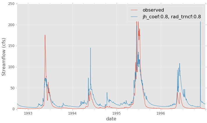
Comparison of observed and modeled flow

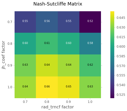
Nash-Sutcliffe Matrix of model efficiencies