Command-Line Interface

If you installed using pip, you should now be able to access the PRMS-Python Command-Line Interface (CLI) through the prmspy command. The prmspy CLI is an ongoing work in progress. You can run the prmspy command

prmspy

and you should see the following help message

Usage: prmspy [OPTIONS] COMMAND [ARGS]...

  access PRMS-Python functionality from the command line

Options:
  --help  Show this message and exit.

Commands:
  nash_sutcliffe_matrix  Save a PDF of the Nash-Sutcliffe created from...
  param_scale_sim        Provide params and scaling values; run PRMS...

You can get help messages for the commands by typing them in after prmspy:

prmspy param_scale_sim

prmspy nash_sutcliffe_matrix

Commands

The CLI provides two commands, param_scale_sim and nash_sutcliffe_matrix. They are rather cryptically named, so we will explain these names.

param_scale_sim

param_scale_sim performs a parameter-scaling experiment. The user can pass in any number of parameters and a list of scaling values to use for each parameter. prmspy will modify base parameter data as requested, doing the data management for you, and placing all “scenario” inputs into a UUID4-named directory. prmspy tracks which directories belong to which combination of scaling values, and writes this information on disk in JSON-formatted metadata saved to the same parent directory as the scenario input and output data.

Below is an example using prmspy param_scale_sim to create 121 different scenarios by co-varying two parameters, rad_trncf and snow_adj both across eleven values, 0.5 to 1.5 in 0.1 increments. We provide a title, “Testing prmspy with rad_trncf and snow_adj adjustments”, use eight processors (-n8), run PRMS instead of simply building scenario input data, and write all data to the directory test-run-series.

prmspy param_scale_sim prms_python/models/lbcd \
    -p rad_trncf \
    -s"[0.5, 0.6, 0.7, 0.8, 0.9, 1.0, 1.1, 1.2, 1.3, 1.4, 1.5]" \
    -p snow_adj \
    -s"[0.5, 0.6, 0.7, 0.8, 0.9, 1.0, 1.1, 1.2, 1.3, 1.4, 1.5]" \
    -t"Testing prmspy with rad_trncf and snow_adj adjustments" \
    -n8 \
    -o test-run-series \
    --run-prms

It’s a lot to type in, but it’s actually pretty clear.

What to do with all that data? Move on to the next section to see an option for analyzing the fit of modeled data to observed data as these parameters vary.

nash_sutcliffe_matrix

The Nash-Sutcliffe model efficiency is one of many measures of how well a model output matches known observational data. For this, we are comparing the predicted streamflow matches the observed streamflow.

Mathematically, the Nash-Sutcliffe efficiency (NSE), \(E\) is defined as

\[E = 1 - \frac {\sum_{t=1}^{T}\left(Q_o^t - Q_m^t\right)^2} {\sum_{t=1}^{T}\left(Q_o^t - \overline{Q_o}\right)^2}\]

where for us \(Q_o^t\) is the observed streamflow at time \(t\), \(Q_m^t\) is the modeled streamflow at time \(t\), and \(\overline{Q_o}\) the time average of the observed streamflow.

The Nash-Sutcliffe efficiency can be at most 1 which happens in the unlikely case that the modeled streamflow exactly matches the observed streamflow. The NSE has no lower bound. An NSE of zero means that the time-average would do just as well at predicting the timeseries as the model did. An NSE below zero means that the time-average as a predictor would be a better predictor than the model.

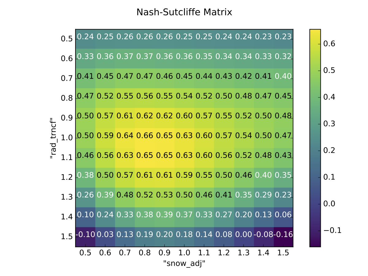
We can calculate a matrix of Nash-Sutcliffe values whose coordinates correspond to combinations of parameter scalings given to prmspy param_scale_sim above.

To build a PDF with a visualization of this image, run the following

prmspy nash_sutcliffe_matrix test-run-series nash-sutcliffe.pdf

Open nash-sutcliffe.pdf and you should see something just like this: